Clustering Analysis
Create signals for analysis
from dtwhaclustering.dtw_analysis import dtw_signal_pairs, dtw_clustering, plot_signals, shuffle_signals, plot_cluster
import numpy as np
from scipy import signal
import matplotlib.pyplot as plt
from dtaidistance import dtw
from scipy.cluster.hierarchy import fcluster

from scipy.cluster.hierarchy import dendrogram
from sklearn.cluster import AgglomerativeClustering

np.random.seed(0)
# sampling parameters
fs = 100   # sampling rate, in Hz
T  = 1      # duration, in seconds
N  = T * fs # duration, in samples
M  = 5      # number of sources
R  = 3      # number of copies
MR = M * R


# time variable
t = np.linspace(0, T, N)

S1 = np.sin(2 * np.pi * t * 7)
S2 = signal.sawtooth(2 * np.pi * t * 5)
S3 = np.abs(np.cos(2 * np.pi * t * 3)) - 0.5
S4 = np.sign(np.sin(2 * np.pi * t * 8))
S5 = np.random.randn(N)

time_series = np.array([S1, S2, S3, S4, S5])

fig, ax = plot_signals(time_series)
plt.show()
Add noise and make 3 copies of each signal
SNR = 0.2
X0 = np.tile(S1, (R, 1)) + np.random.randn(R, N) * SNR
X1 = np.tile(S2, (R, 1)) + np.random.randn(R, N) * SNR
X2 = np.tile(S3, (R, 1)) + np.random.randn(R, N) * SNR
X3 = np.tile(S4, (R, 1)) + np.random.randn(R, N) * SNR
X4 = np.tile(S5, (R, 1)) + np.random.randn(R, N) * SNR
X = np.concatenate((X0, X1, X2, X3, X4))
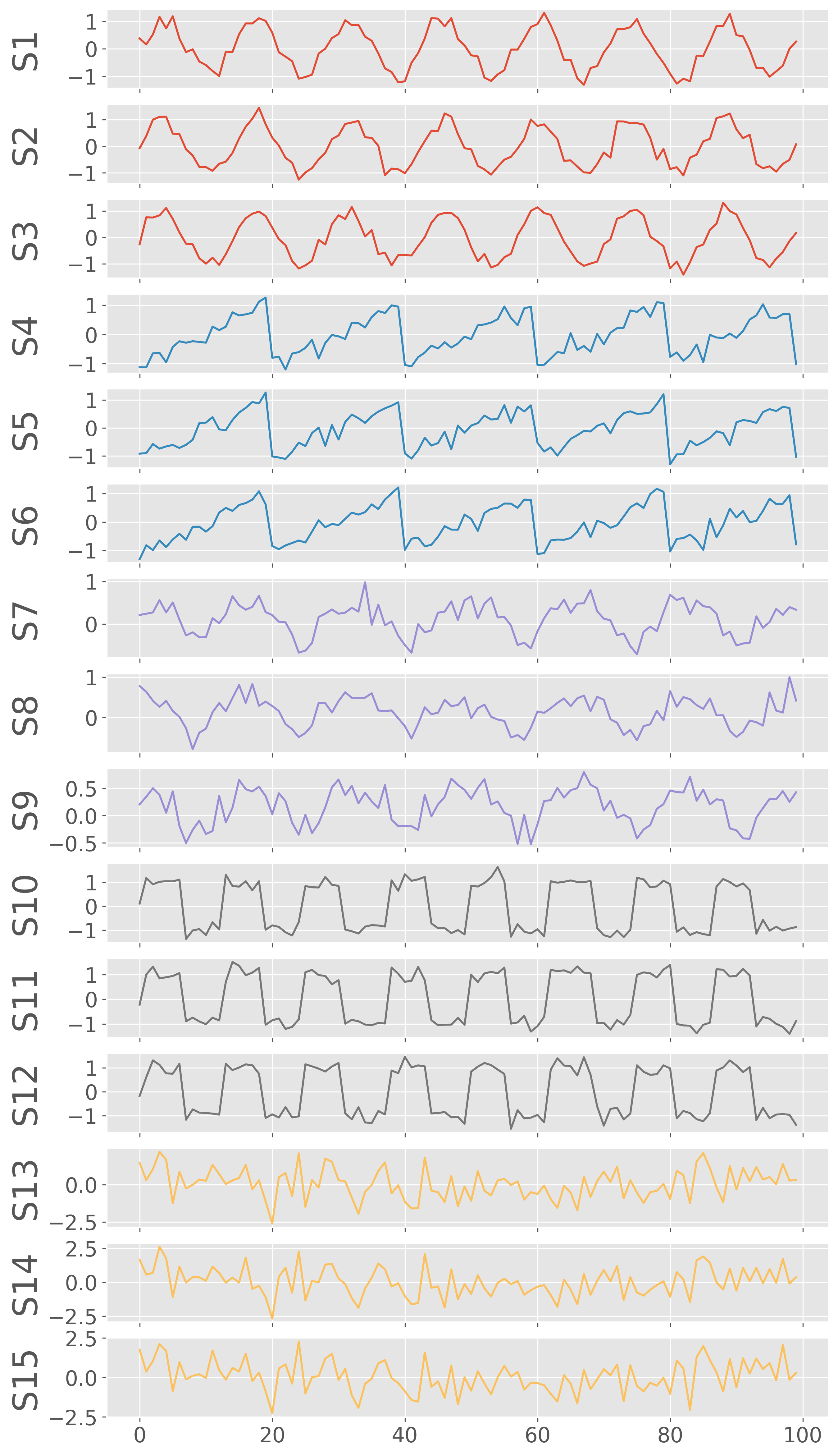
color = ['C0']*3+['C1']*3+['C2']*3+['C3']*3+['C4']*3
fig, ax = plot_signals(X,figsize=(10,20), color=color)
plt.show()
Geographically distribute the signals
Now, we have 15 signals in total. Let us also randomly make these signals distributed in geographical space by assigning them longitudes and latitudes. We assume that the signals with similar waveforms are geographically co-located.
S0 variants (S0, S1, S2) -> xrange(0-3) yrange(7-10)
S1 variants (S3, S4, S5) -> xrange(1-4) yrange(3-5)
S2 variants (S6, S7, S8) -> xrange(4-8) yrange(4-6)
S3 variants (S9, S10, S11) -> xrange(5-10) yrange(0-4)
S4 variants (S12, S13, S14) -> xrange(5-9) yrange(6-9)
S0_lons = np.random.uniform(0, 3, 3)
S0_lats = np.random.uniform(7, 10, 3)

S1_lons = np.random.uniform(1, 4, 3)
S1_lats = np.random.uniform(3, 5, 3)

S2_lons = np.random.uniform(4, 8, 3)
S2_lats = np.random.uniform(4, 6, 3)

S3_lons = np.random.uniform(5, 10, 3)
S3_lats = np.random.uniform(0, 4, 3)

S3_lons = np.random.uniform(5, 10, 3)
S3_lats = np.random.uniform(0, 4, 3)

S4_lons = np.random.uniform(5, 9, 3)
S4_lats = np.random.uniform(6, 9, 3)

lons = np.concatenate((S0_lons, S1_lons, S2_lons, S3_lons, S4_lons))
lats = np.concatenate((S0_lats, S1_lats, S2_lats, S3_lats, S4_lats))

plot_cluster(lons,lats)
# plt.show()
plt.savefig("signals_locations.pdf", bbox_inches='tight')
Reshuffle the noisy signals
shuffled_idx, shuffled_matrix = shuffle_signals(X, labels=[], plot_signals=False, figsize=(10, 20))
shuffled_lons = lons[shuffled_idx]
shuffled_lats = lats[shuffled_idx]

labels = np.array(['S1a', 'S1b', 'S1c','S2a', 'S2b', 'S2c','S3a', 'S3b', 'S3c','S4a', 'S4b', 'S4c','S5a', 'S5b', 'S5c'])
newlabels = labels[shuffled_idx]

color = np.array(color)
color = color[shuffled_idx]
fig, ax = plot_signals(shuffled_matrix,figsize=(10,20), color=color, labels=newlabels)
plt.savefig("shuffled_signals.pdf", bbox_inches='tight')
Cluster reshuffled signals
dtw_cluster2 = dtw_clustering(shuffled_matrix, labels=newlabels, longitudes=shuffled_lons, latitudes=shuffled_lats)
dtw_cluster2.plot_dendrogram(annotate_above=3,xlabel="Signals", figname="example_dtw_cluster.png",distance_threshold="optimal")
In the above dendrogram, we manually selected the threshold distance to be 3 to find the best clusters
Plot the geographical locations of the clusters
dtw_cluster2.plot_cluster_xymap(dtw_distance=3, figname=None, xlabel='', ylabel='', fontsize=40, markersize=200, tickfontsize=30, cbarsize=40)
plt.savefig("signals_cluster_xy_map.pdf", bbox_inches='tight', edgecolors='black', linewidths=5)
Polar dendrogram
kwargs_dendro={
"plotstyle":'seaborn',
"linewidth":5,
"gridwidth":0.8,
"gridcolor":'gray',
'xtickfontsize':60,
'ytickfontsize':60,
"figsize":(40,40),
"distance_threshold":"optimal" #use optimal number of clusters estimated by elbow method
}

dtw_cluster2.plot_polar_dendrogram(**kwargs_dendro)
plt.savefig("example_polar_dendro.pdf", bbox_inches='tight')
How the DTW distance changes with iterations to obtain the dendrogram?
dtw_cluster2.plot_hac_iteration()
plt.show()
dtw_cluster2.plot_optimum_cluster(legend_outside=False)
plt.savefig("optimum_clusters.pdf", bbox_inches='tight')
Euclidean distance-based cluster
def compute_linkage(model):
    # create the counts of samples under each node
    counts = np.zeros(model.children_.shape[0])
    n_samples = len(model.labels_)
    for i, merge in enumerate(model.children_):
        current_count = 0
        for child_idx in merge:
            if child_idx < n_samples:
                current_count += 1  # leaf node
            else:
                current_count += counts[child_idx - n_samples]
        counts[i] = current_count

    linkage_matrix = np.column_stack([model.children_, model.distances_,
                                    counts]).astype(float)
    return linkage_matrix

def plot_dendrogram(model, **kwargs):
    # Create linkage matrix and then plot the dendrogram

    linkage_matrix = compute_linkage(model)

    # Plot the corresponding dendrogram
    dendrogram(linkage_matrix, **kwargs)


#‘ward’ minimizes the variance of the clusters being merged
model = AgglomerativeClustering(distance_threshold=0, n_clusters=None, affinity='euclidean',linkage='ward')

model = model.fit(X)

plt.figure(figsize=(20, 8))
# plot the top three levels of the dendrogram
plot_dendrogram(model, p=5, color_threshold=5)
plt.xticks(fontsize=26)
plt.yticks(fontsize=26)
plt.axhline(y=5, c='k')


plt.xlabel("Signal Indexes")
plt.savefig('example_euclidean_cluster.pdf',bbox_inches='tight')
plt.close()
Both Euclidean and DTW based clustering results are similar. However, we can see some obvious differences. Let us list some of the similarity and differences for the above example.
Both the results found 5 significant clusters.
Both Euclidean and DTW based HAC found that the random function based time series (12, 13, 14) are most dissimilar
The two closest clusters with DTW is sawtooth (6,7,8) and sine func(0,1,2). While that with the Euclidean, it is abs_cosine (6,7,8) and sawtooth fn (3,4,5)
The two results are similar because the signals considered for this example are stationary in nature.